Directional Coupler

Introduction

Directional couplers (DC) are an important category of optical splitters. They are typically composed of two adjacent single-mode waveguides, and the coupling coefficient is determined by both the length of the coupler and the spacing between them. This feature allows for effective control of the splitting ratio.

When it comes to directional couplers, we pay close attention to several key parameters, including insertion loss, splitting ratio, device dimensions, and operating bandwidth.

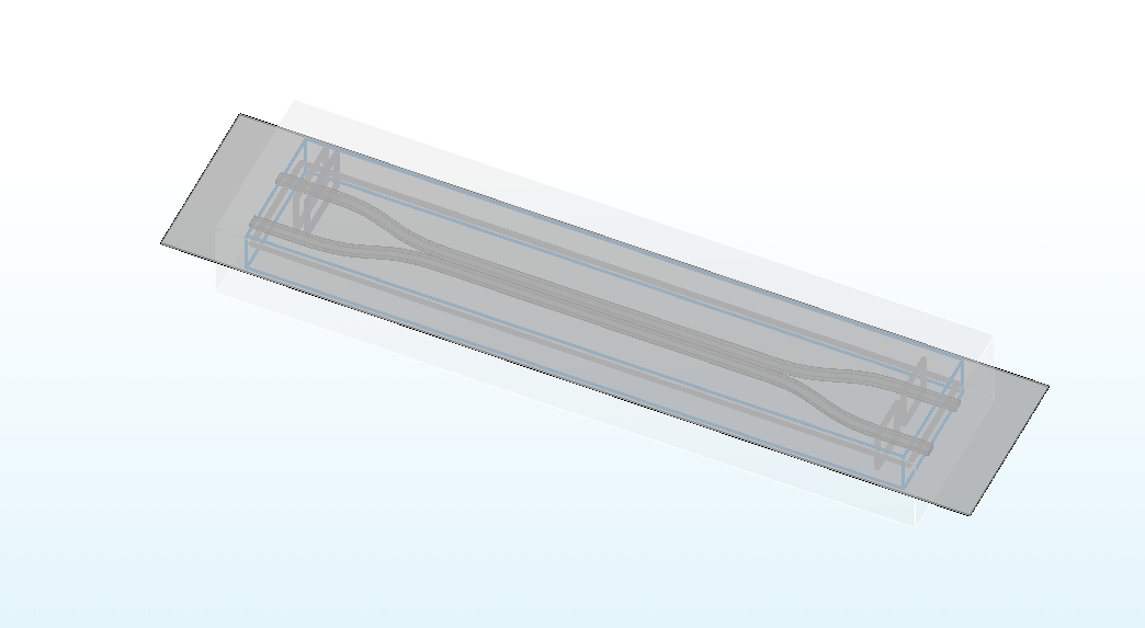Simulation Methods

The FDE module can be used to calculate the symmetric and anti-symmetric mode field distributions of the directional coupler’s two arms. From these calculations, the effective index can be determined, allowing for the theoretical calculation of the coupling length required to achieve the target splitting ratio.

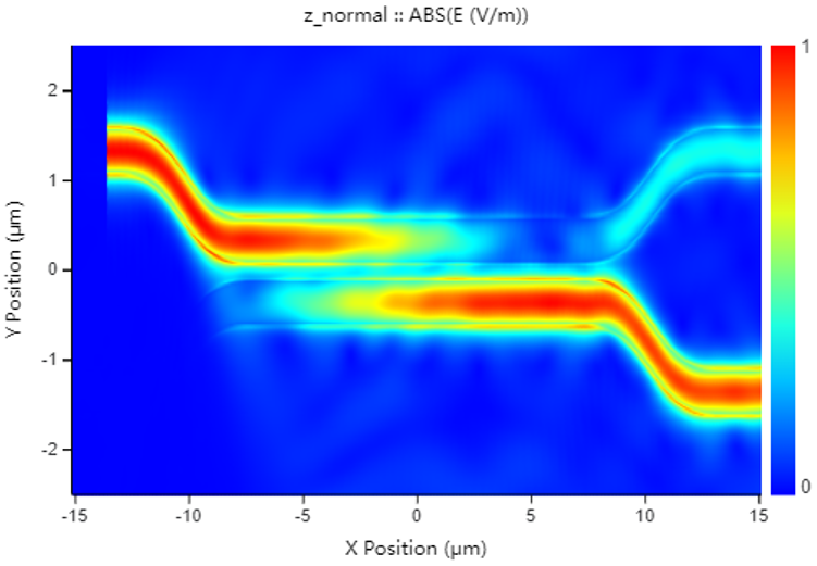
And the FDTD module can be used to perform precise calculations of light propagation in the DC. The light field transmission images in the monitor allow for a visual assessment,the related data of which facilitate further optimization and validation of the coupling length and spacing parameters in the DC splitter.

After data processing, it can be obtained that the splitting ratio, insertion loss, and operating bandwidth of DC. In designing high-performance directional couplers for various optical communication and integrated photonics applications, these calculations and optimization processes are instrumental.

Directional Coupler(FDE module)

Using the FDE module, we will calculate symmetric and antisymmetric modes in a Directional Coupler modeled with the SDK. The input light can be considered a combination of the symmetric mode and the antisymmetric mode so that we can precisely calculate the coupling coefficient by effective index from the FDE module. Referring to the Silicon Photonics Design written by Lukas Chrostowski, we build the structure of the Directional coupler in the simulation.

1. Basic Operations

1.1 Import File

Once you have installed and configured the environment, import the python code and the GDS layout. The example library and related model code are usually located in the directory :examples/func_demo. The GDS file is generally imported into the path :examples/examples_gds

1.2 SDK Initialization

Create a new terminal and run the code after you import the python script and GDS file. Max-Optics SDK may take some time to connect the service.

2. Code Description

Now let's learn the meaning of functions and parameters that correspond to the code.

2.1 import Modules

To begin, we need to use the import command to call the relevant functional modules. For instance, we import the typing , os and time module in python. At the same time ,we import the customized module maxoptics_sdk.all and maxoptics_sdk.helper.

from typing import List, Literal, NamedTuple
import os
import time
import maxoptics_sdk.all as mo
from maxoptics_sdk.helper import timed, with_path

The typing module provides support for type hints and annotations, which are used to indicate the expected types of variables, function arguments, and return values in your code.
The os module provides a way to use operating system-dependent functionality such as reading or writing to the file system, working with environment variables, and executing system commands.
The time module provides various functions to work with time-related operations and to measure time intervals.
The maxoptics_sdk package provides all in one optical simulation with Python.

2.2 Define Simulation

Firstly, We define parameters and give them a default value, such as the simulation wavelength and grid accuracy. Note that we can override this value in the following code.

def simulation(*, run_mode="local", wavelength =1.55, grid = 0.02, number_of_trial_modes = 20, run_options: "RunOptions", **kwargs, ):

The provided code contains comments that define the simulation parameters. Let's explain each of these parameters.
The function simulation is used to define the simulation parameters for the program.
The run_mode parameter determines the type of calculation resources to be used.
The wavelength parameter specifies the wavelength of the input light in micrometers.
The grid parameter represents the grid accuracy in micrometers.
Lastly, the number_of_trial_modes parameter sets the number of modes to be calculated.
The **kwargs is a special syntax used in function definitions to accept an arbitrary number of keyword arguments as a dictionary.

2.3 Define Parameters

Define commonly used parameters in this region, such as the width and height of the simulation boundary, the start time of the simulation, the path and name for the simulation output, the path to the imported GDS layout, and other parameters required for structural parameterized modeling.

# region --- General Parameters ---
yspan_solver = 5
zspan_solver = 2
time_str = time.strftime("%Y%m%d_%H%M%S", time.localtime())
path = kwargs["path"]
simu_name = f"FDE_DC_yspan={yspan_solver}_{time_str}"
gds_file_root_path = os.path.abspath(os.path.join(path, ".."))
gds_file = gds_file_root_path + "/examples_gds/DC.gds"
project_name = f"{simu_name}_{run_mode}"
plot_path = kwargs.get("plot_dir", path) + "/plots/" + project_name + "/"
kL = [f"0{k}" for k in range(5)]
export_options = {"export_csv": True, "export_mat": True, "export_zbf": True}
l_bend = 5.6  # the length of z bend
l_beam = 15  # the length of 2 beams
l_input = 2.5  # the length of input wg
# endregion

The code defines several parameters and variables necessary for the simulation process. The yspan_solver parameter represents the width of the simulation boundary specified in micrometers. Similarly, the zspan_solver parameter denotes the height of the simulation boundary in micrometers. The time_str variable is used to obtain the current time as a timestamp for the simulation.
The path variable defines the file path for the simulation, while simu_name specifies the name of the simulation file.
The gds_file_root_path variable defines the path for importing the GDS layout.
The project_name variable assigns a name to the project for the simulation output.
The plot_path variable determines the directory where the simulation result plots will be saved.
The export_options parameter allows for the definition of options for exporting the simulation results.
Lastly, the variables l_bend ,l_arm, and l_input represent the lengths of specific components within the simulation, such as the length of the z-bend, the length of the two arms, and the length of the input waveguide, respectively.
These parameters and variables together facilitate the successful execution and organization of the simulation process.

2.4 Define Materials

Indeed, let's proceed to the next step, where we set up the materials required for the simulation in this region. In this case, we will directly use relevant materials from the MO material library.

# region --- Material ---
mt = pj.Material()
mt.add_lib(name="Si", data=mo.Material.Si_Palik, order=2)
mt.add_lib(name="SiO2", data=mo.Material.SiO2_Palik, order=2)
mt.add_lib(name="Air", data=mo.Material.Air, order=2)
# endregion

The add_lib is used to define three parameters name,data and order.
The data calls up the property of simulation materials in the MO material library.
The Order parameter determines the mesh order for the material during the simulation.
Besides, we also support users to customize the material with add_nondispersionfunction.

2.5 Create Model

Next, we will create the Directional Coupler model. We have two options for modeling the structure:

# region --- Structure ---
st = pj.Structure()
st.add_geometry(name="box", type="gds_file",
                property={"general": {"path": gds_file, "cell_name": "TOP", "layer_name": (1, 1)},
                            "geometry": {"x": 0, "y": 0, "z": 0.11, "z_span": 6},
                            "material": {"material": mt["SiO2"], "mesh_order": 1},},)
st.add_geometry(name="dc",type="gds_file",
                property={"general": {"path": gds_file, "cell_name": "TOP", "layer_name": (0, 0)},
                            "geometry": {"x": 0, "y": 0, "z": 0.11, "z_span": 0.22},
                            "material": {"material": mt["Si"], "mesh_order": 2},},)
st.add_geometry(name="slab",type="Rectangle",
                property={"geometry": {"x_min": -l_input - l_bend - l_beam / 2 - 3, "x_max": l_input + l_bend + l_beam / 2 + 3,
                                        "y": 0, "y_span": 8, "z": 0.045, "z_span": 0.09,},
                            "material": {"material": mt["Si"], "mesh_order": 2},},)
# endregion

Here, we import the DC layout from the GDS file. we can create the DC model directly within the SDK using the Structure function.
The name parameter defines the structure name.
The type parameter specifies the structure type.
The path, cell_name, and layer_name parameters point to the GDS file and specify the relevant layers and cell names used in the layout.
The geometry parameter sets the structure's coordinates.
The material parameter specifies the material properties
The mesh_order parameter sets the mesh order for building structures.

2.6 FDE Simulation

After establishing the model, we can add the simulation region. We add the FDE simulation module to support mode calculations and frequency scans. We can also and define the simulation boundary conditions. This involves specifying the geometry of the simulation region, the boundary conditions in the xyz directions, and detailed parameters.

# region --- Simulation ---
simu = pj.Simulation()
simu.add(name=simu_name,type="FDE",
            property={"background_material": mt["SiO2"],
                    "geometry": { "x": 0, "x_span": 0, "y": 0, "y_span": yspan_solver, "z": 0, "z_span": zspan_solver, },
                    "boundary_conditions": { "y_min_bc": "PEC", "y_max_bc": "PEC", "z_min_bc": "PEC", "z_max_bc": "PEC", },
                    'general': {'solver_type': '2d_x_normal'},
                    "mesh_settings": {"mesh_refinement": { "mesh_refinement": "curve_mesh" },
                                        "mesh_factor": 1.2, "global_mesh_uniform_grid": { "dy": grid, "dz": grid, },},},)
simu_res = simu[simu_name].run()
# endregion

In this code segment, the name parameter defines the name of the simulation module.
The general parameter specifies the type of the simulation module within the structure. It supports the following list selection['2d_x_normal','2d_y_normal','2d_z_normal'].
The mesh_settings parameter is set to the previously defined the mesh.

In this case,we use Perfect Electric Conductor(PEC) boundary condition. The PEC boundary condition is a modeling approach used to simulate the behavior of perfectly conducting surfaces or boundaries in electromagnetic wave propagation analyses. This effectively models the behavior of a material with infinite conductivity and perfect electrical shielding. This boundary condition is particularly relevant when dealing with the interaction of light and electromagnetic fields with highly conductive materials, such as metals.
Moreover, We also provide the usual boundary condition like Perfectly Matched Layer(PML) and Perfect Magnetic Conductor (PMC), you can change the PEC to PML or PMCof 4 dimensions in the code.

2.7 Add Sub-mesh

To achieve more accurate calculations of the model's modal fields, we can add a sub-mesh.

# region --- Sub Mesh ---
lm = pj.LocalMesh()
lm.add(name="sub_mesh",
        property={"general": {"dx": 0.002, "dy": 0.002, "dz": 0.002},
                    "geometry": { "x": 0, "x_span": 6, "y": 0, "y_span": 2, "z": 0, "z_span": 0.2,},},)
# endregion

In this code segment, we use the LocalMesh to add a sub-mesh.
The name parameter defines the name of the mesh.
The general parameter specifies the grid accuracy in the xyz directions (in this case, 0.002 micrometers in each direction).
The geometry parameter sets the coordinates of the sub-mesh.

2.8 Add Analysis

Such as mode expansion and frequency analysis, we can add a sub-mesh to achieve more analysis.

# region --- Analysis ---
analysis = pj.Analysis()
analysis.add_analysis(name="Mesh Structure", type="FDEAnalysis",
                        props={"workflow_id": simu_res.workflow_id, "simulation_name": "FDE",
                                "modal_analysis": {"calculate_modes": run_options.run, "mesh_structure": False, "wavelength": wavelength,
                                                "number_of_trial_modes": number_of_trial_modes,"search": "max_index", "n": 1,
                                                "calculate_group_index": False,
                                                "bent_waveguide": { "bent_waveguide": False, "radius": 1, "orientation": 0, "location": "simulation_center", },},
                                "frequency_analysis": {"frequency_analysis": run_options.run_frequency_sweep,
                                                    "start_wavelength": 1.50, "stop_wavelength": 1.60,
                                                    "number_of_points": 3, "effective_index": 2.67,
                                                    "detailed_dispersion_calculation": False, }, } )
# endregion

The wavelength parameter sets the wavelength-related parameters for the simulation.
The search parameter specifies the mode search type. It supports the following list selection['near_n','max_index'].
In this case, we use max_index to automatically search for the mode with max index in the structure. To use the ‘near_n’, we need to set the data in ‘n’.
The bent_waveguide parameter can be used to set parameters for a bent waveguide.
The frequency_analysis parameter allows us to set parameters for frequency scans or mode calculations with varying wavelengths.

2.9 Retrieve Results

In this region, you can retrieve and store the simulation results.

# region --- Run ---
result_fde = analysis["Mesh Structure"].run()
if run_options.run:
        k = kL[2]
        res = result_fde.extract(data="calculate_modes",
                                    savepath=f"{plot_path}{k}_neff_table",export_csv=True,)
        print(res.to_string(index=False))
        for m in range(len(res)):
            k = kL[3]
            result_fde.extract(data="calculate_modes", savepath=f"{plot_path}{k}_mode{m}",
                                attribute="Ey", real=True, imag=False, mode=m, show=False, **export_options,)

if run_options.run_frequency_sweep:
        k = kL[4]
        result_fde.extract(data="frequency_analysis", savepath=f"{plot_path}{k}_freq_sweep_neff",
                            attribute="neff", real=True, imag=True, show=False, export_csv=True, export_mat=True,)
return project_name
# endregion

The extract function allows you to extract specific simulation results and store them for further analysis.
The attribute parameter specifies the type of simulation results to be extracted.
The mode parameter corresponds to the index of the FDE calculation mode.
The real and imag parameters are used to extract the real and imaginary parts of the simulation results, respectively.
If you run the frenquency sweep to calculate mode at different wavelength, you can also extract the relevant results. As an example above, we extrat the effective index.

2.10 Switches

In this section of the code, the simulation function is called and executed, which allows you to reset relevant parameters for more convenient parameter scanning and optimization design. We also support control switches for various functionalities at the end of the code, and you can use configuration flags(True or False). These flags can be used to turn specific functionalities on or off, making it easier to check the model and perform efficient calculations.

class RunOptions(NamedTuple):
    index_preview: bool
    run: bool
    run_frequency_sweep: bool
    extract: bool

if __name__ == "__main__":
    simulation(run_mode="local", wavelength=1.55, grid=0.02,
               number_of_trial_modes=3, run_options=RunOptions(index_preview=True, run=True, run_frequency_sweep=True, extract=True),)

By turning on/off the relevant functionalities, you can control the simulation process and obtain the desired results. For example, the index_preview is to control whether to output images of the structural refractive index. run determines whether to run the program. run_frequency_sweep is used to enable frequency scanning, and extract is used to control data extraction. Properly utilizing these switches can help you inspect the simulation effectively.

3. Output Results

2. The results of the calculation mode will be stored in a CSV format file for subsequent data processing in Python and Excel.

mode_order	TE ratio	neff_real	neff_imag	ng_real	ng_imag	wavelength(nm)	loss(dB/cm)
0	0.986860	2.593169	0	0	0	1550	0
1	0.987740	2.542372	0	0	0	1550	0
2	0.941287	2.129843	0	0	0	1550	0

1. Image of the Ey electric field component intensity in symmetric and antisymmetric mode modes.

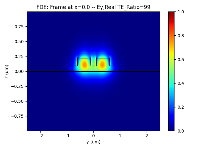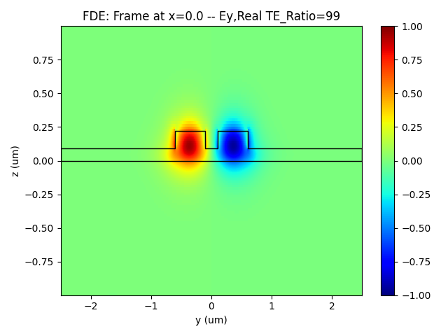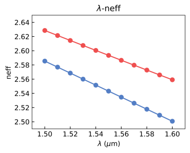
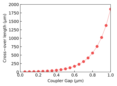
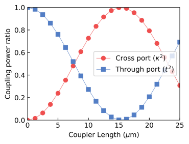
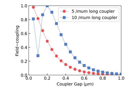
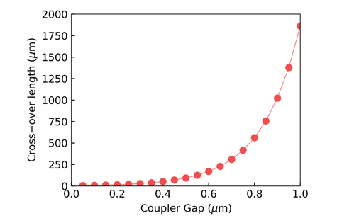
2. According to the effective refractive index of the obtained mode field, Python is used for data processing and drawing.

 The coupling length under the gap between two waveguides is calculated with the formula:

$$L_x = \frac{\lambda}{2|neff_1-neff_2|}$$

 We can also get the coupling coefficient by the formula:

$$\kappa = |sin(\frac{\pi\delta(n)L}{\lambda})|$$

5. Similarly, we can obtain the relationship between the gap (distance) between two waveguides and the coupling coefficient and the relationship between the wavelength and the coupling length.

Directional Coupler(FDTD module)

Next, we will learn how to model a Directional Coupler using the SDK and calculate the light propagation in the structure using the FDTD module.

1. Basic Operations

Similarly, after installing and configuring the environment, we import the relevant python code file and the GDS layout for the model. The example library and related model code are typically stored in the directory examples/func_demo, and the GDS file is imported into the folder examples/examples_gds.

2. Code Description

Next, we will continue to learn about the specific functionalities corresponding to the code.

2.1 Define Parameters

Like the operations with the FDE module, after configuring the simulation wavelength, grid precision, and other parameters, we need to set the relevant parameters for simulation and parameterized modeling. This includes defining the paths and names for the simulation files and output results and specifying the path for importing the GDS layout.

# region --- General Parameters ---
l_bend=5.6 # the length of z bezier bend
l_beam=15 # the length of 2 beams
l_input=2.5 # the length of input wg
monitor_w = 3.0
monitor_h = 2.0
waveform_name = "wv" + str(round(wavelength * 1000))
time_str = time.strftime("%Y%m%d_%H%M%S", time.localtime())
path = kwargs["path"]
simu_name = "FDTD_DC"
project_name = f'{simu_name}_{time_str}'
plot_path = f'{path}/plots/{project_name}/'
gds_file_root_path = os.path.abspath(os.path.join(path, '..'))
gds_file = gds_file_root_path + "/examples_gds/DC.gds"
# endregion

2.2 Define Materials

Subsequently, we ues the materials required for the simulation. We also support users to specify the refractive indices of Si (Silicon) and SiO2 (Silicon Dioxide) materials.

# region --- Material ---
mt = pj.Material()
mt.add_lib(name='Si', data=mo.Material.Si_Palik, order=2)
mt.add_lib(name='SiO2', data=mo.Material.SiO2_Palik, order=2)
mt.add_lib(name="Air", data=mo.Material.Air, order=2)
# endregion

The add_nondispersion function adds a non-dispersion material to the project in the simulation.
The data, is specified as a list, typically in the format [(index real, index imag)]. This list contains the complex refractive index values for the material, enabling the simulation to model its optical properties accurately.
The function allows users to incorporate non-dispersion materials into the simulation, contributing to a comprehensive and precise optical analysis of the system under investigation.

2.3 Define Waveform

In this region, we define the parameters relevant to the wavelength.

# region --- Waveform ---
wv = pj.Waveform()
wv.add(name=waveform_name,type='gaussian_waveform',
       property={'set': 'frequency_wavelength',  # selections are ['frequency_wavelength','time_domain']
                 'set_frequency_wavelength': {
                        'range_type': 'wavelength',  # selections are ['frequency','wavelength']
                        'range_limit': 'center_span',  # selections are ['min_max','center_span']
                        'wavelength_center': wavelength,
                        'wavelength_span': wavelength_span,},})
# endregion

The Waveform function is used to retrieve the waveform manager for the current project. It allows users to access and manipulate the waveform sources used in the simulation.
The name parameter specifies the name of the waveform source.
The wavelength_center parameter defines the center of the wavelength range for the source.
The wavelength_span parameter determines the span of the wavelength range for the source.

2.4 Create Model\Boundary

Next, similar to the procedure in the FDE module, we create the model by importing the GDS layout.

# region --- Structure ---
st = pj.Structure()
st.add_geometry(name="box",type="gds_file",
                property={"general": {"path": gds_file,"cell_name": "TOP","layer_name": (1, 1)},
                          "geometry": {"x": 0, "y": 0, "z": 0.11, "z_span": 6},
                          "material": {"material": mt["SiO2"], "mesh_order": 1}},)
st.add_geometry(name="dc",type="gds_file",
                property={"general": {"path": gds_file,"cell_name": "TOP","layer_name": (0, 0)},
                          "geometry": {"x": 0, "y": 0, "z": 0.11, "z_span": 0.22},
                          "material": {"material": mt["Si"], "mesh_order": 2}},)
st.add_geometry(name='slab',type='Rectangle',
                property={'geometry': {'x_min': -l_input-l_bend-l_beam/2-3,'x_max':l_input+l_bend+l_beam/2+3,'y': 0,'y_span': 8,'z': 0.045,'z_span': 0.09},
                          'material': {'material': mt['Si'], 'mesh_order': 2},} ,)
# endregion

2.5 FDTD Simulation/local mesh

Next, we add the FDTD simulation and detailed parameters for the boundary condition. Additionally,we can set the sub-mesh for improved precision.

# region --- Simulation ---
simu = pj.Simulation()
simu.add(name=simu_name,type="FDTD",
         property={"background_material": mt["SiO2"],
                   "geometry": {"x": 0,"x_span": 2*(l_input+l_bend+l_beam/2-0.5),"y": 0,"y_span": 6,"z": 0.11,"z_span": monitor_h},
        "boundary_conditions": {"x_min_bc": "PML", "x_max_bc": "PML", "y_min_bc": "PML", "y_max_bc": "PML", "z_min_bc": "PML", "z_max_bc": "PML",
                                           "pml_settings": {"all_pml": {"layers": 8, "kappa": 2, "sigma": 0.8, "polynomial": 3, "alpha": 0, "alpha_polynomial": 1, }}},
        "general": { "simulation_time": 10000, },
        "mesh_settings": {"mesh_factor": 1.2, "mesh_type": "auto_non_uniform",
                          "mesh_accuracy": {"cells_per_wavelength": grids_per_lambda},
                          "minimum_mesh_step_settings": {"min_mesh_step": 1e-4},
                          "mesh_refinement": { "mesh_refinement": "curve_mesh", } },},)
# endregion

# region --- Sub Mesh ---
lm = pj.LocalMesh()
lm.add(name="sub_mesh",
       property={"general": {"dx": 0.05, "dy": 0.02,"dz": 0.02 },
                 "geometry": {"x": 0, "x_span": 2*(l_input+l_bend+l_beam/2-0.5), "y": 0, "y_span": 6, "z": 0.11, "z_span": monitor_h },},)
# endregion

The Simulation manager is critical for setting up and running simulations in the current project.
The name parameter allows users to assign a unique name to the simulation for identification purposes.
The type parameter defines the type of the simulation.
we define the boundary conditions for the simulation using the boundary dictionary, where the x ,y and the z directions all have PML boundary conditions.The simulation_time parameter specifies the duration of the simulation.
The mesh_settings parameter enables users to configure various settings related to the simulation mesh. The mesh_accuracy parameter controls the precision of the mesh used in the simulation.
The cells_per_wavelength parameter determines the wavelength precision used in the simulation.
The minimum_mesh_step_settings parameter sets the minimum mesh step, allowing users to define the smallest allowable size for mesh elements.
Users can tailor the simulation setup to meet their requirements by utilizing these input parameters, enabling accurate and efficient electromagnetic simulations of complex optical structures.

2.6 Source

Then we need to establish the light source in the input waveguide, as shown below.

# region --- ModeSource ---
src = pj.Source()
src.add(name="source",type="mode_source",
        property={"general": {"mode_selection": "user_select",
                              "waveform": {"waveform_id": wv[waveform_name]}, "inject_axis": "x_axis", "direction": "forward"},
                  "geometry": {"x": -l_input-l_beam/2-l_bend+2, "x_span": 0, "y": 1.35, "y_span": monitor_w, "z": 0.11, "z_span": monitor_h },
                  "modal_analysis": {"mode_removal": {"threshold": 0.01}} ,})
# endregion

The Source function is utilized to retrieve the source manager for the current project.
The type parameter specifies the type of the source and is formatted as either ["mode_source"] or ["gaussian_source"].
The name parameter represents the name assigned to the source.
The inject_axis parameter defines the axis of the source.
The property parameter allows for defining specific properties associated with the source.

2.7 Monitor

In this region, we set up the monitors.

# region --- Monitor ---
mn = pj.Monitor()
mn.add(name="Global Option", type="global_option",
       property={"frequency_power": {"spacing_type": "wavelength", "spacing_limit": "center_span",
                 "wavelength_center": wavelength, "wavelength_span":wavelength_span, "frequency_points": 3},},)
mn.add(name="z_normal",type="power_monitor",
       property={"general": {"frequency_profile": {"wavelength_center": wavelength, "wavelength_span": wavelength_span, "frequency_points": 3,},},
                 "geometry": {"monitor_type": "2d_z_normal", "x": 0, "x_span": 2*(l_input+l_bend+l_beam/2-0.5), "y": 0, "y_span": 5, "z": 0.11, "z_span": 0},},)
mn.add(type="power_monitor", name="input_reflect",
       property={"general": {"frequency_profile": {"wavelength_center": wavelength, "wavelength_span": 0.1, "frequency_points": 11}},
                 "geometry": {"monitor_type": "2d_x_normal",
                              "x": -l_input-l_beam/2-l_bend+1.5, "x_span": 0, "y": 1.35, "y_span": monitor_w, "z": 0.11, "z_span": monitor_h },})
mn.add(type="power_monitor",name="through",
       property={"general": {"frequency_profile": {"wavelength_center": wavelength, "wavelength_span": 0.1, "frequency_points": 11}},
                 "geometry": {"monitor_type": "2d_x_normal",
                              "x": l_input+l_beam/2+l_bend-2,"x_span": 0, "y": 1.35, "y_span": 2, "z": 0.11, "z_span": monitor_h },},)
mn.add(name="cross",type="power_monitor",
       property={"general": {"frequency_profile": { "wavelength_center": wavelength, "wavelength_span": 0.1, "frequency_points": 11 }},
                 "geometry": {"monitor_type": "2d_x_normal",
                              "x": l_input+l_beam/2+l_bend-2, "x_span": 0, "y": -1.35, "y_span": 2, "z": 0.11, "z_span": monitor_h },})
# endregion

For the global monitor, the Monitor function is utilized to retrieve the monitor manager for the current project, which allows users to access and manage various types of monitors used during simulation.
The name parameter represents the name of the Global Option associated with the monitor.
The type parameter defines the type of the Global Option and is formatted as a list containing one of several monitor types. The property parameter is used to define and set the relevant parameters specific to the chosen monitor type. These parameters control the monitor's behavior and data collection settings during the simulation.

The power monitor is a configuration setting that allows users to specify various simulation parameters.
The name parameter assigns a name to the power monitor.
The type parameter defines the type of power monitor.
The general parameter pertains to settings related to the frequency domain and frequency-dependent behaviors of the simulation.
The geometry parameter is used to define the geometric characteristics of the simulated structure.

2.8 Preview Source Mode

To calculate the input mode light and save its electric field intensity data.

# region --- Calculate Mode ---
if run_options.calculate_modes:
    simu[simu_name].preview_modes(source_name = "source",
                                  savepath=f"{plot_path}00_source_modeprofile_fdeonly",
                                  attribute="E", real=True, imag=True, mode=0, show=False, export_csv=True, )
# endregion

2.9 Run Simulation

Then, we run the simulation. 

# region --- Run ---
if run_options.run:
    fdtd_res = simu[simu_name].run(
        resources={"compute_resources": "gpu", "gpu_devices": [{"id": 0},{"id": 1}]})
# endregion

2.10 Analysis

In this region, we run the analysis for the simulation. The mode_expansion parameter involves relevant settings for mode expansion simulations. Users can customize the simulation settings by utilizing these input parameters to achieve accurate and comprehensive results based on their specific simulation requirements.

# region --- ModeExpansion ---
analysis = pj.Analysis()
analysis.add(name="me_through",type="mode_expansion",
             property={"workflow_id": fdtd_res.workflow_id,
                       "mode_expansion": {"direction": "positive", "monitors_for_expansion": [ {"name": "me_through", "frequency_monitor": "through"} ],
                                          "mode_calculation": {"mode_selection": "user_select", "mode_index": [0, 1, 2, 3],
                                                               "override_global_monitor_setting": {"wavelength_center": wavelength, "wavelength_span": 0.1,
                                                                                                    "frequency_points": 11,},},},})
analysis.add(name="me_cross",type="mode_expansion",
             property={"workflow_id": fdtd_res.workflow_id,
                       "mode_expansion": {"direction": "positive", "monitors_for_expansion": [ {"name": "me_cross", "frequency_monitor": "cross"} ],
                       "mode_calculation": {"mode_selection": "user_select", "mode_index": [0, 1, 2, 3],
                                            "override_global_monitor_setting": {"wavelength_center": wavelength, "wavelength_span": wavelength_span,
                                                                                "frequency_points": 11, },},},})
me_res1 = analysis["me_through"].run()
me_res2 = analysis["me_cross"].run()
# endregion

2.11 Results

The codes below is uesd to extract the results.

# region --- See Results ---
if run_options.extract and run_options.run:
    for λ in [1.5, 1.55, 1.6]:
        fdtd_res.extract(data="fdtd:power_monitor", savepath=plot_path + "01_top_profile" + str(λ) + "um",
                         monitor_name="z_normal", target="intensity", attribute="E", real=True, imag=True,
                         wavelength=str(λ), plot_x="x", plot_y="y", show=False, export_csv=True,)
        fdtd_res.extract(data="fdtd:power_monitor", savepath=plot_path + "01_monitorThrough_modeprofile_fdtd_"+ f"{wavelength}" + "um",
                         monitor_name="through", target="intensity", attribute="E", real=True, imag=False,
                         wavelength=f"{wavelength}", plot_x="y", plot_y="z", show=False, export_csv=True,)
        fdtd_res.extract(data="fdtd:power_monitor", savepath=plot_path + "02_Trans_ThroughVsLambda_power",
                         monitor_name="through", target="line", attribute="T", real=True, imag=False,
                         plot_x="wavelength", show=False, export_csv=True,)
        me_res1.extract(data="fdtd:mode_expansion", savepath=plot_path + "021_ME_ThroughVsLambda_mode",
                        target="line", attribute="T_forward", real=True, imag=True,
                        monitor_name="through", mode_expansion_name="me_through", mode=0, plot_x="wavelength", show=False, export_csv=True,)
        fdtd_res.extract(data="fdtd:power_monitor", savepath=plot_path + "01_monitorcross_modeprofile_fdtd_"+ f"{wavelength}" + "um",
                         monitor_name="cross", target="intensity", attribute="E", real=True, imag=False,
                         wavelength=f"{wavelength}", plot_x="y", plot_y="z", show=False, export_csv=True,)
        fdtd_res.extract(data="fdtd:power_monitor", savepath=plot_path + "02_Trans_crossVsLambda_power",
                         monitor_name="cross", target="line", attribute="T", real=True, imag=False,
                         plot_x="wavelength", show=False, export_csv=True,)
        me_res2.extract(data="fdtd:mode_expansion", savepath=plot_path + "021_ME_crossVsLambda_mode",
                        target="line", attribute="T_forward", real=True, imag=True, monitor_name="cross", mode_expansion_name="me_cross",
                        mode=0, plot_x="wavelength", show=False, export_csv=True,)
# endregion

2.12 Switches

At the end of all codes, We control the switches of various functional modules.

class RunOptions(NamedTuple):
    index_preview: bool
    calculate_modes: bool
    run: bool
    extract: bool

if __name__ == "__main__":
    simulation(wavelength=1.55, wavelength_span=0.1 , grids_per_lambda=6,
               run_options=RunOptions( index_preview=True, run=True, calculate_modes=True, extract=True),)

3. Output Results

After running the program, we can obtain a series of corresponding output results:

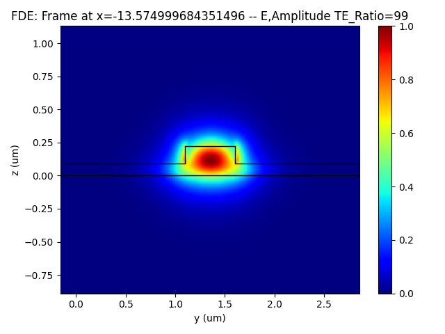
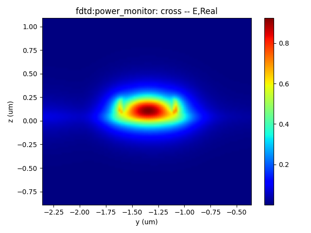
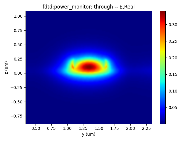
1. Incident light electric field intensity, CRO output port electric field intensity, and TRU output port electric field intensity.

2. DC (Directional Coupler) Z-direction electric field intensity at different wavelengths: 1.50 μm, 1.55 μm, and 1.60 μm.

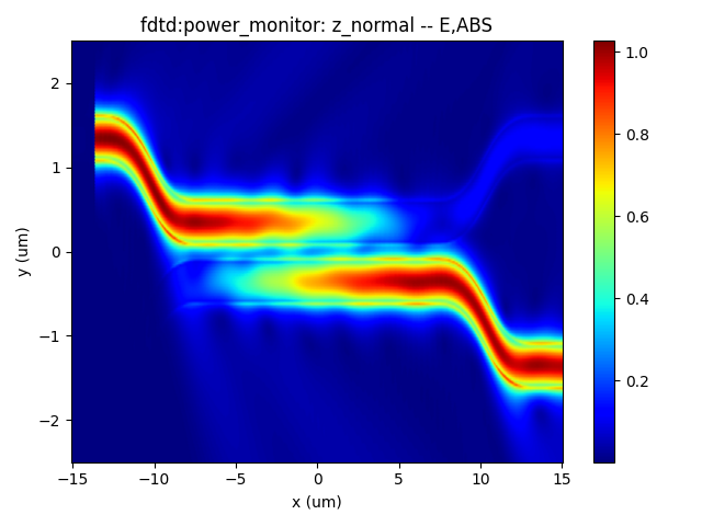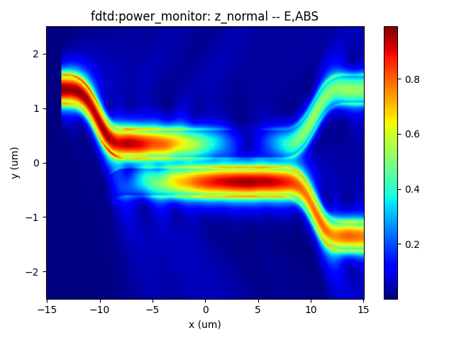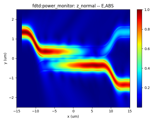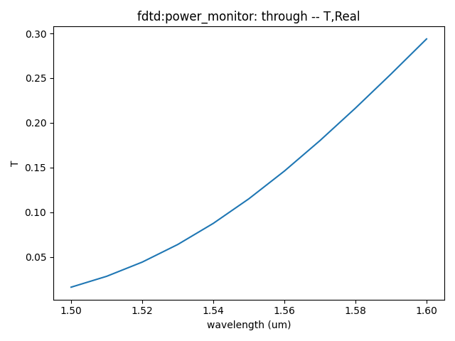
1. Cross output port and TRU output port transmittance at different wavelengths,from 1.50 μm to 1.60 μm.

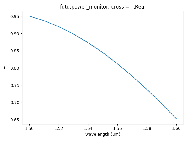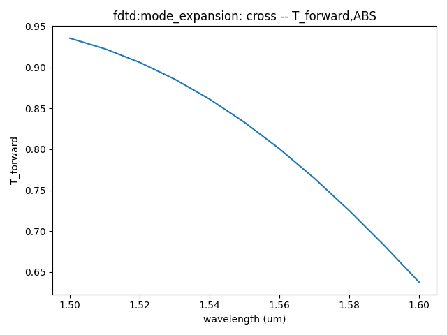
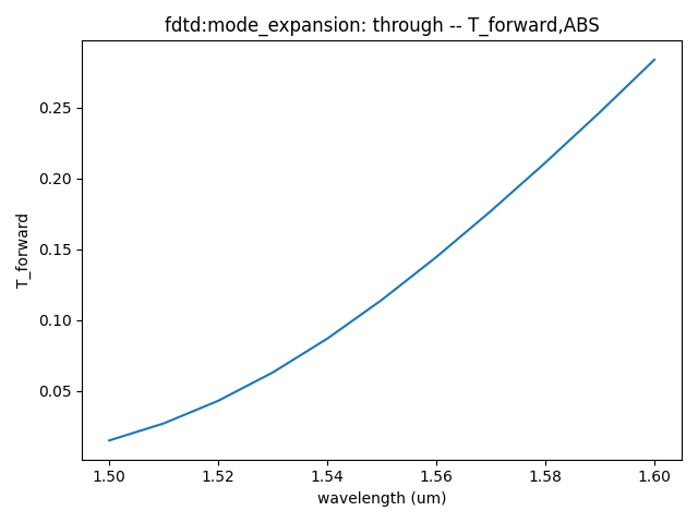
4. TE0 mode transmittance at Cross output port and TRU output port for different wavelengths,,from 1.50 μm to 1.60 μm.

Based on the information provided, we can get the following results when propogating wavelength is 1.55 μm and the two arm length of directional couper is equal to 15 μm: 1. Insertion Loss: 0.236 dB; 2. Power Split Ratio: 11.2 : 83.3 (or approximately 11.2% to one port and 82.8% to the other port); 3. Dimensions: Approximately 5 μm X 25 μm.

Supplement

To view a function's definition and supported parameters or a parameter dictionary, you can right-click on its name and select "Go to Definition" or press "Ctrl" while left-clicking on its name to view its definition, showing the available parameters and their descriptions.

References

Chrostowski, L., & Hochberg, M. (2015). Silicon Photonics Design: From Devices to Systems. Cambridge: Cambridge University Press. doi:10.1017/CBO9781316084168